Race is a defining part of political identity in the United States, and so it should be no surprise that accurately modeling race can be beneficial for many political campaign activities. For instance, many organizations work to improve turnout in specific communities of color, or want to target persuasion on a given issue to certain racial group. Alternatively, race and ethnicity might be desired as an input to a larger voting or support likelihood model, given that race is generally predictive of both voting likelihood and candidate support.
Unfortunately, complete self-reported race data is only available in 7 states, where it is required by law: Alabama, Florida, Georgia, Louisiana, Mississippi, North Carolina, and South Carolina. Pennsylvania and Tennessee also have an optional field on voter registration forms. Outside of these states, race and ethnicity need to be collected individually, or modeled. These models commonly take advantage of the name (especially surname) of the individual voter, and other information in the voter file to do so.
In this post, I’ll explore a Bayes’ rule based method for modeling racial identity, and how it can be extended with additional information from state voter files where available. Obviously, it won’t be as predictive as something like Catalist or Civis Analytics’ ones (which have the benefit of huges swathes of additional survey and other data, not to mention more sophisticated modeling), but it can help illustrate the benfits and limitations of such tools. In the next posts, I’ll explain how natural language processing models can achieve still higher accuracy by extracting more information from names themselves. Since the Florida voter file has self-reported race data and is easy to access, we’ll test our models’ effectiveness against that ground truth.
A simple first method
The census surname files are a an incredible source of information on how race correlates with names, and are the starting point of our model. In these files, the census provides race percentage breakdowns for any surname with more than 100 occurrences in the United States, except where redacted for privacy reasons. The data is available only aggregated at the national level. In practice, this means coverage of about 90% of the population.
For many voters, surname is the only information we need to make an accurate classification: names such as Carlson, Meyer, and Hanson are in excess of 90% white, with similar surnames existing for other races. Unfortunately, many names aren’t as clear cut, and some names like Chavis are less than 40% likely to be any race. This is a good starting point, but we can do better.
As our first improvement, Elliot et al. (2009) incorporates census geolocation (county, tract, or block) data, using Bayes’ theorem.
Bayes’ theorem is a natural way to integrate the new census evidence we have, updating our initial beliefs with more data. P(A) and P(B) are the probabilities of events A and B occurring independently of each other, and P(A \vert B) and P(B \vert A) are conditional probabilities, such as the probability a given voter is white given their surname, or P(white \vert surname). Bayes’ theorem appears in it’s simplest form below, giving us an updated probability utilizing the new information:
P(A|B) = \frac{P(B|A) P(A)}{P(B)}
Of course, we’re interested in integrating multiple pieces of evidence (surname/geolocation for now, with more coming later), and applying it to multiple voters. The equations will be much more involved, but remember that we’re essentially just extending the above equation to work with multiple inputs, over multiple voters. Note that I’ll be using the notation from Imai and Khanna (2016), which is somewhat clearer than the notion from Elliot et al.
We want P(R_i = r \vert S_i = s, G_i = g), the conditional probability that the voter i belongs to the racial group r given their surname s and geolocation g. R, S, and G are the sets of all racial groups, all surnames, and all geolocations respectively. Thus, as a final expression we’ll get:
P(R_i = r \vert S_i = s, G_i = g) = \frac{P(G_i = g \vert R_i = r) P(R_i = r|S_i = s)}{\sum_{r'\in R} P(G_i = g|R_i = r) P(R_i = r|S_i = s) }
We already have almost all these probabilities between the census surname list and census demographic data. P(R_i = r \vert S_i = s) is the racial composition of surnames from the surname list. But what about P(G_i = g \vert R_i = r)? As an intermediate step, we first need to calculate P(G_i = g \vert R_i = r) , which we can calculate using Bayes’ rule again. P(G_i = g \vert R_i = r) is then \frac{P(R_i = r \vert G_i = g) P(G_i = g)} {\sum_{r'\in R} P(R_i = r \vert G_i = g') P(G_i = g)}, completing everything we need to produce our second model.
This model, like the surname list, produces probabilistic predictions of race, for instance, a given voter is 94.3% likely to be white, given their name and geolocation. The probabilities sum to 1 across the races.
We’ll get to how to use and evaluate such models soon, but first: given that we’ve started to include information from the voter file to improve our predictions, why don’t we use other fields we have such as age, party registration, and gender? They all are likely to contain some conditional information about a voter’s race, and while party registration isn’t reported in every state, it is in Florida.
That’s exactly the proposal of Imai and Khanna (2016), and it works well. The equations get slightly more complicated, but extending Bayes’ rule to include more and more variables doesn’t change all that much. We have to calculate more intermediate probabilities, but the essential process and reasoning of incorporating new information to update our belief is the same. If you want to see the full model written out, with space for an arbitrary number of new variables X_i, you can find it in the linked paper.
Use and Evaluation
Now that we have a probability distribution over the racial groups, how do we utilize them?
We might take the highest probability race and use that as our prediction. Alternatively, as an input in a later model, we might choose to simply incorporate all 5 probabilities, allowing our following model as much information as possible about the racial identity of a voter. Catalist, the democratic data vendor, turns probabilities into simple categories such as “likely white” or “possibly black”, which simplify working with the results on a campaign.
As a final idea, we might have an application in mind where you want to only predict a certain race when you’re very confident in your prediction. For example, you might be hoping to target a turnout mailer written in Spanish to only Hispanics, and as few non-Hispanics as possible. To do this, we’d utilize only high probability predictions- say, above 85% likely to be Hispanic. By changing that threshold, you could optimize the size of your mail universe versus the specificity and efficiency of it, finding the best balance for your campaign.
As our last example showed, when utilizing such probabilistic predictions, there is naturally an accuracy tradeoff involved in selecting what type of threshold to use. We could misleadingly say our model is extremely accurate if we only use a high threshold, but a fairer, more systematic evaluation would require looking at how it preforms over multiple such thresholds. That’s what we’ll develop next: Area Under the Curve (AUC), a systematic method for evaluating classifiers.
There are 4 possible outcomes to making a classification: a True Positive (TP), False Positive (FP), True negative (TN), and False Negative (FN). As an example then, a true positive is when we predicted positive, and the ground truth label was actually positive.
Rather than building a table of these 4 outcomes, called a confusion matrix, we’ll be working with summary statistics of these outcomes. The True Positive Rate (or sensitivity or recall) is \frac{TP}{TP+FN}. In other words, out of all the points that are (ground truth) positive, how many did we correctly classify? Similarly, the False Positive Rate is \frac{FP}{FP+TN}. High True Positive Rate is good: it means we’ll miss relatively few positive examples. On the other end of things, low False Positive Rate is what we want: it means fewer negative points will be misclassified.
By calculating these two statistics at a variety of thresholds, then plotting a curve with the FPR on the x-axis and TPR on the y-axis, we can get a deeper understanding of the tradeoff. This is called an Receiver Operating Characteristic. Given what I’ve said about the meaning of the TPR and FPR, can you figure out quality of the 3 classifiers that are graphed below?
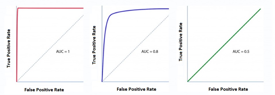 The first is a perfect classifier: at all tradeoff points, it has a TPR of 1, and FPR of 0. The second is pretty good: at most tradeoff points it does well. The third, a straight line from (0, 0) to (1,1) is a random classifier: it’s equivalent to guessing.
As an overall summary then, the area under this curve (AUC) is of our one number summary of these graphs. The shown classifiers have AUC 1, .8, and .5 respectively.
Results
Now that we’ve built up a relatively complex model, and learned how to use and evaluate it, let’s plot some ROC curves, and look at AUCs for our models.
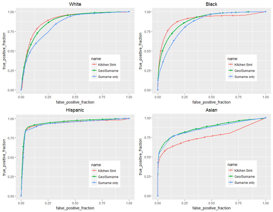
And here’s the AUC table: bold is the highest overall for each race.
| White | Black | Hispanic | Asian | |
|---|---|---|---|---|
| Surname | 0.8414369 | 0.8562679 | 0.9325489 | 0.8606716 |
| Geo/Surname | 0.8792853 | 0.8918873 | 0.9492531 | 0.8717517 |
| Kitchen Sink | 0.8903922 | 0.8979003 | 0.9362794 | 0.7648270 |
Looking at these, there are a lot of interesting patterns!
White: The White models’ results are perhaps what we most expected. With more data, each subsequent model does better, and the overall result is strong.
Black: Interestingly, the kitchen sink model still does the best overall with black voters, but by a much smaller margin than with whites. Also, once the true positive rate gets to around .90, curves cross! This is a good illustration of the importance of plotting ROC curves when doing classification- depending on your campaign, you might correctly choose either the Geo/Surname model or the Kitchen Sink one, depending on what type of cutoff you need.
Hispanic: The Hispanic models are all very close together: with surname information being so effective in classifying Hispanics (more effective than any model for the other races), there isn’t much room for census or voter file data to improve things.
Asian: These models are significantly weaker than all the others, but still reasonable. The unexpected trend though, is that the kitchen sink model preforms much worse than the other two. Given how few Asian voters there are overall in Florida, this downturn is probably explained by the relatively low density of any Asians across the other inputs, like age, sex, or party. Thus, while geographic information might slightly improve things, Floridians are so unlikely to be Asian overall that all of those extra variables don’t carry any useful information about who might be Asian.
Overall, these Bayes’ Theorem models have a lot of attractive features. While the predictiveness of names, and what variables you have from the voter file might vary state to state, the models can used anywhere in the US. They’re also quite a strong baseline for accuracy as well- far, far better than random, even for Asian voters. Unlike models we’ll discuss in the next post, these models require no training data. Finally, they’re transparent- if you want to check how surname, geolocation, and party weighed in to a particular decision, it’s only a few calculations with Bayes’ rule away.
Of course, we’d love higher accuracy, and we can get there with natural language processing. What about those ~10% of voters whose name aren’t in the census surname file? If a name starts with “Mc”, but isn’t in the census surname list, I personally would guess they’re of Irish descent, and therefore white. And what about using first names, middle names, and name suffixes? It’s linguistic patterns like these that we’ll hope to exploit with NLP, in the next post.
You can find the code used to write this post here.
Reuse
Citation
@online{timm2018,
  author = {Timm, Andy},
  title = {Predicting Race Part 1- {Bayes’} Rule Method and Extensions},
  date = {2018-04-10},
  url = {https://andytimm.github.io/posts/Race Models Pt 1/race_models_part1.html},
  langid = {en}
}